Other Projects

A Few Interesting Class Projects

Adaptive Feedback Linearization Control of Planar Bipedal Robot

Class Project for Intelligent Control Systems Course: EE-5322; Fall, 2017

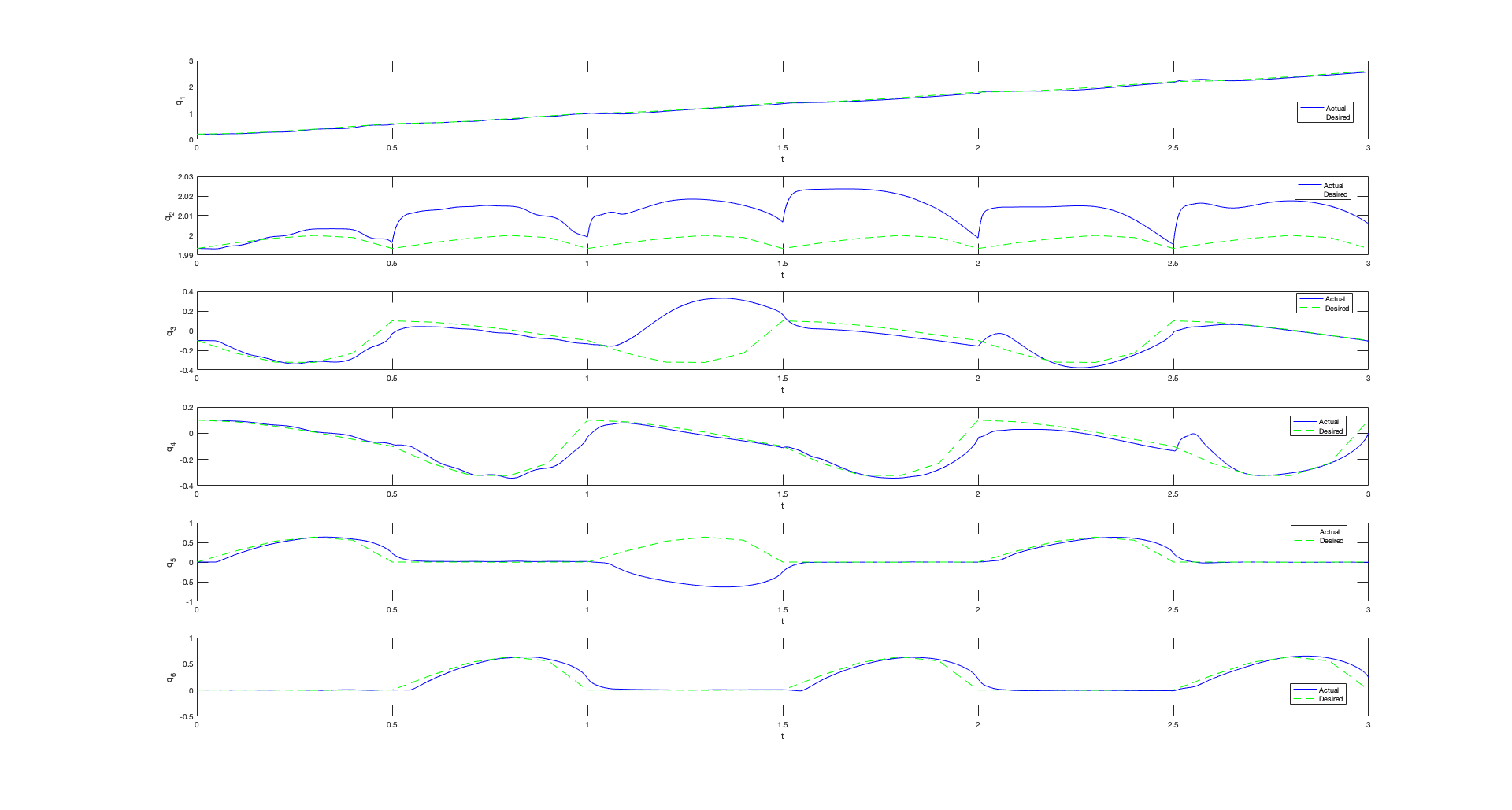
The goal of this project was to implement an adaptive feedback linearization control strategy for the legged locomotion of a bipedal robot. The bipedal robot model used for this project was a simple stick-figure planar model of 6 degrees of freedom, consisting of a base and two legs. The end-points of these legs were considered to be the feet of the robot that came in and out of contact with the ground. The contact between the robot feet and the ground were assumed to be not slipping or rebounding at any time. The degrees of freedom of this system changes depending upon the contact states of the two feet. Hence, the plant dynamics for the robot has different modes depending upon the contact states at the two feet, thereby yielding what is known as a hybrid dynamic system. It is very difficult to control hybrid dynamic systems with a linear controller without an inverse dynamics model. Therefore, in this project the idea of using adaptive controller to linearize the plant dynamics was explored for this problem. Adaptive controllers use the outputs of the system as regression functions and scale them with certain weighing parameters to yield a model for the inverse plant dynamics. These weighing parameters are then updated with the help of the system's error dynamics based on a recursive least-squares approach. The adaptive inverse plant model obtained using this appproach is then cascaded with the actual plant model to yield an apparent linearized plant model, which can be controlled using a simple linear proportional controller. The reference input to the system was calculated from operation space desired trajectories by means of inverse kinematics using a levenberg-marquardt approach. The figure below shows the animation of the biped model and also shows a comparison between the desired configuration space trajectories vs. actual trajectories.

Although initially, when I conceived this idea of using an adaptive controller on a biped robot model as my class project, I wanted to implement it on a more realistic, underactuated model of biped. However, eventually I found out that adaptive feedback linearization of underactuated system can be quit complicated and would have been way beyond the scope of my class project. So I ended up changing the model to a fully-actuated one. Nevertheless, I found this topic very interesting, and would like to explore this more in future.

Minimum-Time Path Planning for 2-Robot Obstacle Avoidance and Randezvous Problem

Class Project for Optimal Control of Dynamic Systems Course: ME-5335; Fall, 2016

The objective of this project was to develop a minimum-time path planning and obstacle avoidance algorithms for a 2-Robot (Unmanned Ground Vehicles) rendezvous problem. The dynamics for the UGV robots used for this problem were given by simple kinematic model: $$ \begin{array}{ccl} \dot{x_r} & = & V \cos(\phi) \sin(\theta) \\ \dot{y_r} & = & V \cos(\phi) \cos(\theta) \\ \dot{\theta} & = & \frac{V}{L} \sin(\theta) \end{array} $$ where \(x_r\), \(y_r\) and \(\theta\) are the position coordinates and heading angle for a robots, \(V = 0.2\) units and \(L\) are the constant velocity and width of the robot respectively. \(\phi\) is the steering angle and also the control input to the system. The steering angle (contol) is bounded by the inequality: \(-\frac{\pi}{2} \leq \phi \leq \frac{\pi}{2}\).

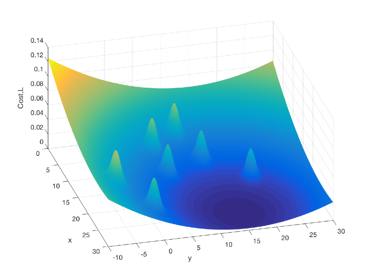
The path-planning required for this problem was posed as a dynamic optimization problem, and an objective functional (Lagrangian) was formulated which combined two cost terms: 1) a cost term directly proportional to the distance between the robots and the goal, and 2) a cost term inversely proportional to the exponential of the distance between the robots and the obstacles. The figure above shows an example of the cost function with respect to a given robot position. The Lagrangian functional was augumented with a set of lagrange multipliers to formulate a hamiltonian function, which was then used to derive the necessary conditions for optimaility (by means of calculus of variations), which yielded a two-point boundary value problem (TPBVP). Finally, in order to get a minimum-time path a shooting method algorithm based on a cost function on the final time was developed to get the solution. The animation below shows the minimum-time path and the control history for this problem.

Note that this is probably not the best approach for solving this type of minimum-time randezvous problem. Direct solution methods such as differential inclusion or collocation are probably better suited for faster solution to this type of problem. Nevertheless, I chose this approach because I find the method of deriving necessary conditions with the help of Calculus of Variations, very elegent and deeply satisfying.

Development and Autonomous Control of Six-Wheeled Skid-Steer Unmanned Ground Vehicle Platform

Class Project for Unmanned Vehicle Development Course: ME-5379; Spring, 2015

Team members: Philip Bailey, Fraiser Jones, Ramakrishna Lanka, Divya Shah

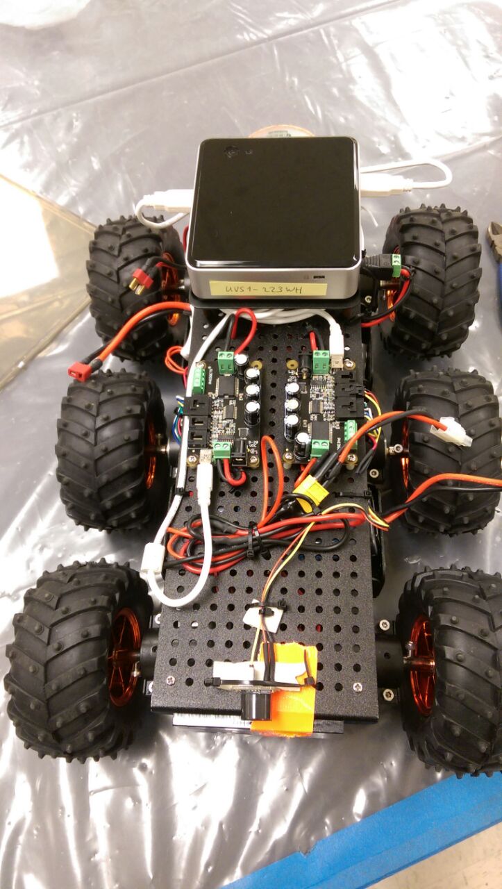
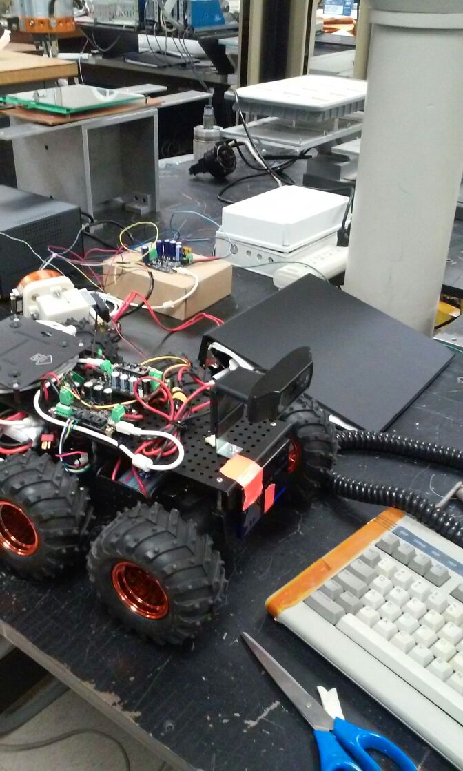
The objective of this project was to develop a completely autonomous Unmanned Ground Vehicle system capable of performing obstacle avoidance and way-point navigation human interference. A six-wheeled differential drive UGV platform was developed by assembling various hobby electronics/robotics parts. The platform was equipped with a number of different sensors viz. GPS, IMU, compass, wheel-encoders, sonar sensor, and camera. An onboard computer (Intel NUC) running MATLAB/Simulink was used to communicate to the low-level micro-controllers and perform the computations for vision, localization, path-planning, guidance and control. The users communicated with the onboard computer via remote desktop and provided high level commands. The MATLAB code running on the computer processed the the video feed from the camera to identify obstacles and goals based on color. A manhattan distance algorithm was used for planning the the path, by assigning way-points, around the obstacles to the goal location. In order to localize the UGV position, the algorithm performed sensor fusion (with inputs from GPS, IMU and wheel-encoder data) by means of Kalman Filtering, based on a skid-steer dynamic model of the robot. The way-points and position estimates were used to calculate desired heading and speed, as part of the guidance for the robot. The guidance portion of the algorithm also utilized the sonar sensor input, as a fail-safe for deflection or halt if the robot goes very close to the obstacles. A PID controller was used to command a desired rpm to the six wheel-motors through a motor-controller.

Reasearch Offshoots

Resultant based multi-polynomial system solver

One of the problems, I was trying to address as part of my work on 3D impact modeling is the resolution of unique slip-directions at the stick-slip transitions, if a point is expected to slip-reverse. Typically,for single-point impacts, this is a very straightforward analysis which boil down to the problem of finding roots of a quadratic, and then choosing the correct solution among them based on an inequality. However, since I was working with multipoint collisions,the problem of finding the slip-direction became a multi-polynomial root finding problem. Note that an important requirement here is to find all possible roots for a given multi-polynomial system, such that the one one them may be selected from them based on a number of inequality criteria. Hence, any recursive root-finding technique wouldn't be applicable here, since they only converge to a single root that depends upon the initial guess. Hence, to solve this problem, I had to look for an alternative method for computing roots, and as a result I came across a number of different methods viz. Homotopy Continuation, Groebner basis, and Resultants. Among these methods, I decided to implement a resultant based approach to solve for the multi-polynomial system roots. Polynomial resultants is actually a very vast subject, typically studied as a part of Algebraic Geometry. I was only concerned about very small proportion of it which offers alternative methods for solving roots simultaneously. The method I ended up implementing is the one that calculates multipolynomial resultants and converts the multipolynomial system to a polynomial eigenvalue problem, such that the roots of the system can be derived from the various eigenvalues and eigenvectors. This approach is suitable for low degree polynomial systems; however for very high-degree this approach doesn't offer good accuracy and is too computationally expensive. Fortunately, the problem I was trying to address only needed roots of degree 4 polynomial system, so this was approach worked pretty well, and was relatively simpler to implement. I tested this algorithm with two problems: (a) inverse kinematics of a 2-bar linkage (this problem can be posed as a root-finding problem for a second degree system of polynomials), and (b) intersection points between multiple 3D elipsoids. The videos below show the solutions obtained by this algorithm.

MultiBody Dynamics Toolbox in MATLAB

I have been working on a Toolbox (library) for performing multibody dynamic simulations on MATLAB. This is going to be based on my research. I am using some of the methods I learned and developed as part of my research to develop this library. I'll probably finish this after my dissertation, then I can include certain parts of my reasearch into this library. I may make it public in future after all the related research get published.

Other Videos